Basic structure

The main structure of the ObsPy library consists of the Trace and the Stream objects, located inside the obspy.core package. The Trace represents a single time series record of seismic data recorded at a single station or sensor. It’s essentially a single waveform with associated metadata (e.g., station code, sampling frequency, component etc.). The Stream is a container of one or more Trace objects. Typically, a Stream contains three recordings or traces: two with horizontal components (e.g., North-South and East-West) and one with a vertical component. Each Trace offers several attributes that provide information about the recording and methods that apply a calculation on the respective recording.

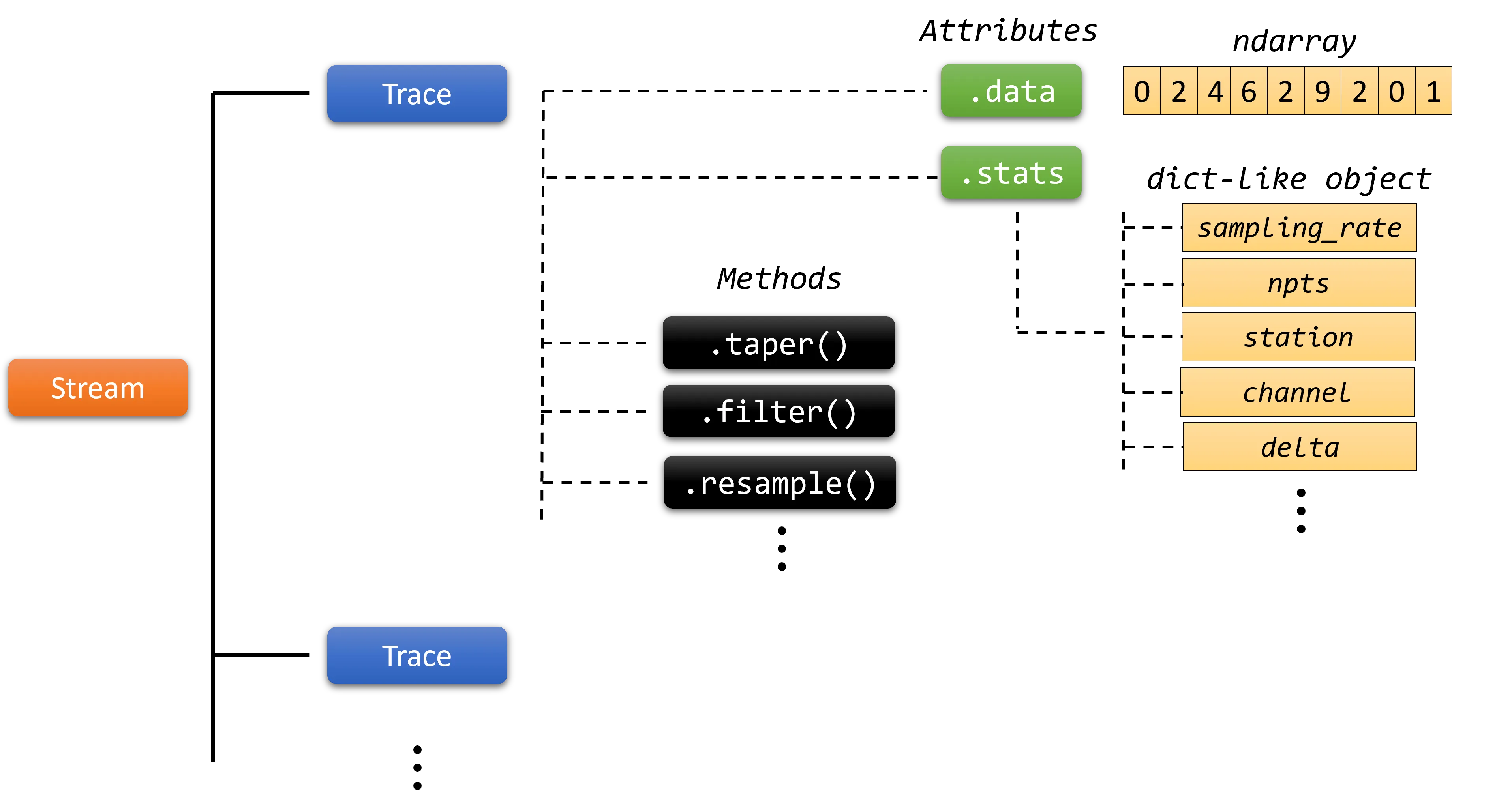The structure of the obspy library. A Stream object consists of one or more Trace objects. Each Trace represents a single waveform or recording and has different methods (.taper(), .filter(), etc.) and attributes (.data, .stats, etc.)

For instance, the .data attribute of a Trace provides its time series data samples and the .stats returns an object that holds metadata or seismic parameters associated with the trace, such as the sampling frequency, date and time of the first data sample, network, station, and other relevant information. In addition, the filter() method, filters the time series data within a specific frequency range and the trim() method cuts the time series to a given start and end time.

ObsPy supports several file formats to read data. One of the most used seimic file format is the MiniSEED format. It is a binary file used to store time series data in a compact and efficient format that includes information about the station, location, timing, and the actual waveform data. MiniSEED files are widely used in seismology and are the standard format for sharing and archiving seismic data.

Before we continue, start by initializing the functions that we will use throughout the rest of the tutorial:

    from obspy.core import read, UTCDateTime, Trace, Stream
    import matplotlib.pyplot as plt
    import pandas as pd

ObsPy Date and Time Manipulation

ObsPy offers extensive support for date and time manipulation. It includes the UTCDateTime object, located at the obspy.core package, to represent date and time. For instance, the start date and the end date of a Trace, which are saved as starttime and endtime in the metadata of a Trace object (generated using the .stats attribute), are both a UTCDateTime data type.

One way to create a UTCDateTime object is by using a Python string:

    # create an ObsPy UTCDateTime object from a Python string
    dt = UTCDateTime("2012-09-07T12:15:00")
    print(dt, type(dt))

    2012-09-07T12:15:00.000000Z <class 'obspy.core.utcdatetime.UTCDateTime'>

You can perform addition, subtraction and extract multiple attributes from this object using the dot notation:

    dt = UTCDateTime("2012-09-07T12:15:00")

    # add 20 seconds
    dt += 20
    print(dt)

    # get some datetime attributes
    print("dt.date -> ", dt.date)
    print("dt.time -> ", dt.time)
    print("dt.year -> ", dt.year)
    print("dt.month -> ", dt.month)
    print("dt.day -> ", dt.day)
    print("dt.hour -> ", dt.hour)
    print("dt.minute -> ", dt.minute)
    print("dt.second -> ", dt.second)
    print("dt.timestamp -> ", dt.timestamp)
    print("dt.weekday -> ", dt.weekday)

    2012-09-07T12:15:20.000000Z
    dt.date ->  2012-09-07
    dt.time ->  12:15:20
    dt.year ->  2012
    dt.month ->  9
    dt.day ->  7
    dt.hour ->  12
    dt.minute ->  15
    dt.second ->  20
    dt.timestamp ->  1347020120.0
    dt.weekday ->  4

Last but not least, one can subtract UTCDateTime objects and get the difference of them in seconds:

    # create two UTCDateTime objects
    dt = UTCDateTime("2012-09-07T12:15:00")
    dt2 = UTCDateTime("2012-09-07T12:20:00")

    # calculate the difference of the two UTCDateTime objects
    diff = dt2 - dt
    print(diff)

    300.0

The starttime and endtime keys in the header information of the recordings need to be in a UTCDateTime data type. Therefore, if you intend to modify these keys within the trace.stats dictionary-like header, convert your datetime string into the UTCDateTime format.

Attributes and Methods

Within ObsPy, you’ll find an array of attributes and methods associated with the Trace class for accessing recording information, seismic file handling, and applying waveform processing techniques. To begin with, utilize the ObsPy read() function to read a file of a recording took place on 04 April, 2014 at 20:08:20 and recorded by CH03 station:

    st = read("20140404_200820_CH03.mseed")
    print(st)

    3 Trace(s) in Stream:
    .CH03..E | 2014-04-04T20:08:20.000000Z - 2014-04-04T20:11:10.000000Z | 100.0 Hz, 17001 samples
    .CH03..N | 2014-04-04T20:08:20.000000Z - 2014-04-04T20:11:10.000000Z | 100.0 Hz, 17001 samples
    .CH03..Z | 2014-04-04T20:08:20.000000Z - 2014-04-04T20:11:10.000000Z | 100.0 Hz, 17001 samples

The file is a MiniSEED file that contains 3 traces or records each with a different component (E, N, Z). We can see the start and the end time of the record, the sampling frequency in Hz and the total samples. Let’s get this information for the first trace of the Stream object:

    # get the first trace
    first_trace = st[0]

    # output the header information of that trace object
    print(first_trace.stats)

    network:
    station: CH03
    location:
    channel: E
    starttime: 2014-04-04T20:08:20.000000Z
    endtime: 2014-04-04T20:11:10.000000Z
    sampling_rate: 100.0
    delta: 0.01
    npts: 17001
    calib: 1.0
    _format: MSEED
    mseed: AttribDict({'dataquality': 'D', 'number_of_records': 34, 'encoding': 'FLOAT64', 'byteorder': '>', 'record_length': 4096, 'filesize': 417792})

We can observe multiple key-value pairs that contain the seismic parameters, such as the station code or name which is CH03, the component of the record which is East-West (E) and the the sampling frequency or sampling rate of 100 Hz. Several other parameters are also apparent like the starting and the ending date of the record (starttime, endtime), the sample distance in seconds (dt), the total number of sample points (npts) and more. The output is a obspy.core.trace.Stats object which is a dict-like object that you can get and set the values.

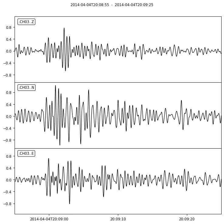
In order to check the traces visually, get the sample data and the time information of the recordings using the .data attribute and the .times() method respectively, and plot them using the Matplotlib Python library.

    # Initialize a matplotlib figure and axes
    # set the figure rows equal to the total number of traces calculated from the length of the stream, len(st)
    fig, ax = plt.subplots(len(st), 1)

    # Loop through all the traces in the stream object (st)
    for n, tr in enumerate(st):
        # get the time information of the current trace
        xdata = tr.times()

        # get the data of the current trace
        ydata = tr.data

        # plot the graph with legend, the trace channel or component
        ax[n].plot(xdata, ydata, label=tr.stats.channel)

        # add the legend on the plot
        ax[n].legend()

    # adjust the subplots so that they do not overlap
    plt.tight_layout()

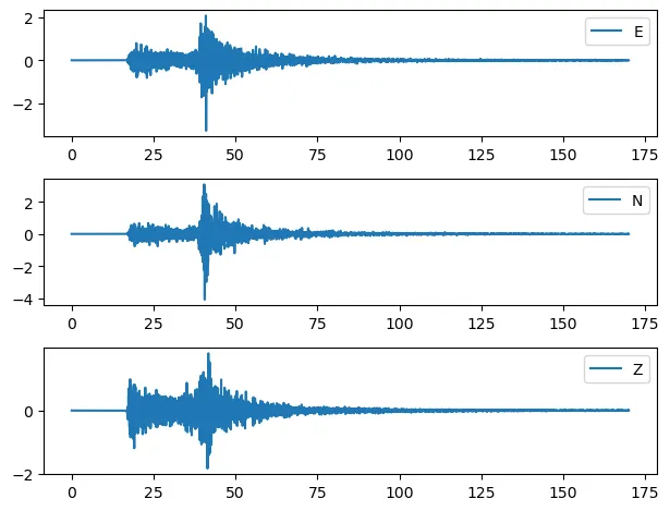Recordings of the MiniSEED file plotted using the matplotlib library

We could achieve a similar result by just using the st.plot() method of the Stream object (st):

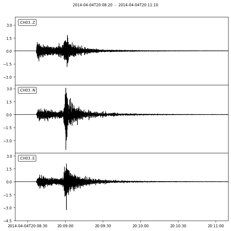Recordings of the MiniSEED file plotted using the .plot() method of the stream object

This method can get some parameters to control the styling of the plots such as the color of the waveforms, the size of the plot, the rotation and size of the x axis labels and more.

In addition, the Trace object includes several methods that apply a specific calculation on the time series of the recording. For example, apply a bandpass at the previous recording between 1 and 3 Hz using the ObsPy filter() method.

    st.filter('bandpass', fremin=1, fremax=3)

    st.plot()

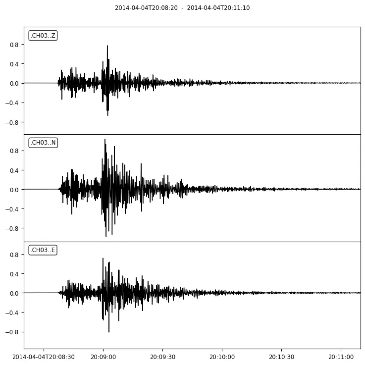Apply a bandpass filter between 1 and 3 Hz at the recording using the ObsPy filter() method

These computations can be applied on the Stream object at once, or at each Trace of the Stream, individually. For instance, trim each recording to get the signal part of the recordings:

    # get the start date of the first record
    startdt = st[0].stats.starttime

    # loop through the traces of the stream and trim each one separately
    for tr in st:
        tr.trim(starttime=startdt+35, endtime=startdt+65)

    st.plot()

Trim the time series to get the signal part

These computations happen inplace on the Stream object. Create a copy of it using the .copy() method to create a new object if you don’t want to change it.

Lastly, save the trimmed Stream object on your local hard drive using the Stream .write() method:

    # save to a file
    st.write('trimmed_mseed.mseed')

Generating Trace and Stream objects from data

In addition to reading seismological files, you have the flexibility to create your own trace and stream from raw data. To create a trace, insert the data values (e.g., acceleration values) as a NumPy ndarray to the data parameter of Trace object, and metadata, at the header parameter as a python dictionary object. Do this for each Trace you want to create. Then, gather all the generated Trace objects into a Python list and pass it into the traces parameter of the Stream class:

    tr1 = Trace(data=np.ndarray(...), header={...})
    tr2 = Trace(data=np.ndarray(...), header={...})
    st = Stream(traces=[tr1, tr2])

We demonstate this by reading a seismic file containing data for three components. This data file includes metadata information positioned at the file’s header, followed by data for each component. Our goal is to read this file and generate a Stream object comprising three individual traces.

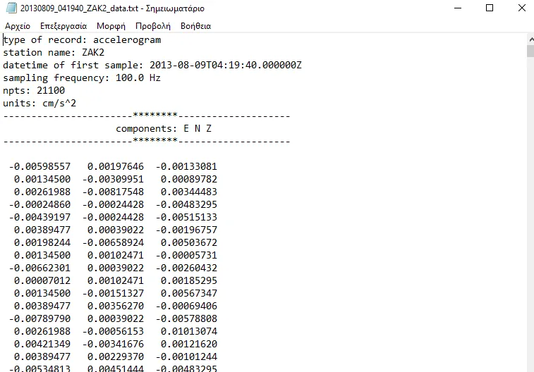Acceleration data in raw ASCII format. The first lines contain the record metadata and the rest of the lines the acceleration data values of the three components

Start by reading the file and collect the file header information in order to build a dictionary of the seismic parameters. Convert the number of points (npts) into a int datatype, the sampling frequency (fs) into a float datatype and the start time of the record (starttime) into a UTCDateTime object. It is important for the keys of the dictionary, to be one of the available options provided in the stats object of the Trace:

    # open the file and read its metadata
    with open('20130809_041940_ZAK2_data.txt') as fr:
        # skip the first line
        fr.readline()

        # read the station name
        station = fr.readline().split(':')[1].strip()

        # read the starting date of the record
        dt_start = fr.readline().split(':', 1)[1].strip()

        # read the sampling frequency in Hz
        fs =  fr.readline().split(':')[1].strip(' Hz\n')

        # read the number of sample points
        npts = fr.readline().split(':')[1].strip()

        # skip 2 lines
        fr.readline()
        fr.readline()

        # read the components
        compos = fr.readline().split(':')[1].split()

    dict_header = {
        "station": station,
        "npts": int(npts),
        "sampling_rate": float(fs),
        "starttime": UTCDateTime(dt_start),
    }

    print(dict_header)

    {'station': 'ZAK2', 'npts': 21100, 'sampling_rate': 100.0, 'starttime': UTCDateTime(2013, 8, 9, 4, 19, 40)}

Then we use the python Pandas library to read the acceleration values of the traces:

    # use the Pandas read-csv method to read the data from text file
    df_data = pd.read_csv('20130809_041940_ZAK2_data.txt', skiprows=10, sep='\s+', header=None)

    # assign the previous components list into the columns
    df_data.columns = compos

At this time we have the metadata and the data of the traces. Using these two parameters, we can create the Trace objects. To do this, loop trough the components, create a header dictionary file for each Trace and add its data:

    # create an empty list to append each trace object
    lt_traces = []

    # then create a trace for each component
    for compo in compos:
        # create a dictionary object and add metadata
        dict_header["channel"] = compo

        # create the trace object
        tr = Trace(data=df_data[compo].to_numpy(), header=dict_header)

        # append the trace into the traces list
        lt_traces.append(tr)

Finally, create the Stream object, from the list of the traces:

    # create the stream by inserting the list of traces into the obspy.core.stream.Stream class
    st = Stream(lt_traces)

    print(st)

    3 Trace(s) in Stream:
    .ZAK2..E | 2013-08-09T04:19:40.000000Z - 2013-08-09T04:23:10.990000Z | 100.0 Hz, 21100 samples
    .ZAK2..N | 2013-08-09T04:19:40.000000Z - 2013-08-09T04:23:10.990000Z | 100.0 Hz, 21100 samples
    .ZAK2..Z | 2013-08-09T04:19:40.000000Z - 2013-08-09T04:23:10.990000Z | 100.0 Hz, 21100 samples

If you require additional information about the ObsPy library, please refer to the documentation.